Head-to-Head Results · Bottle Anomaly Detection

§3 · Results

Head to head

Same photos, same final exam: 126 unseen images, 63 good and 63 defective. Here's the whole story in one table:

	Neural net	PCA
defects caught	62 / 63 (98.4%)	60 / 63 (95.2%)
good bottles wrongly flagged	4 / 63 (6.3%)	6 / 63 (9.5%)
breaks caught	42 / 42 (all)	41 / 42
what it missed	1 contamination	2 contamination + 1 small break

Defects caught, by type

Neural netPCA

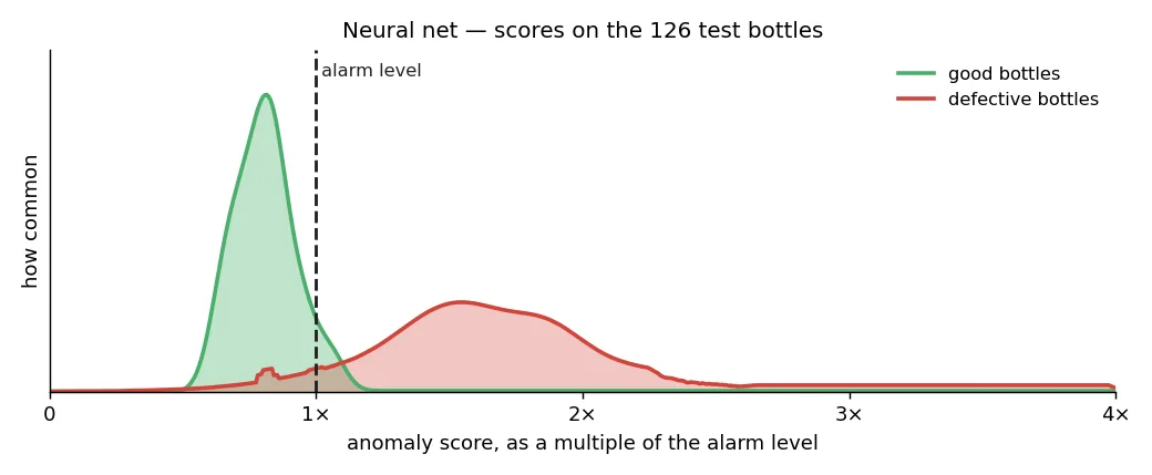
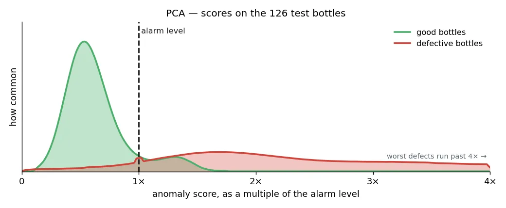
Why the scores work: the two crowds barely touch

Both charts use the same axis: each bottle's score divided by that model's alarm level, so the dashed alarm line sits at 1.0 in both. Good bottles pile up left of the line, defective ones right of it. Where a defect curve leaks left of the line, that's a miss; where a good curve leaks right, that's a false alarm.

Neural net anomaly scores relative to the alarm level — Neural net: only 1 defect leaks left of the line, and 4 good bottles leak right. tap to zoom

PCA anomaly scores relative to the alarm level — PCA: more overlap around the line; its 6 false alarms and 3 misses live there. The worst defects score past 4× the alarm level. tap to zoom

The honest verdict

They're much closer than we expected. The neural net edges it, with two more defects caught, two fewer false alarms and every single break caught, but a well-built PCA gets within a whisker using nothing but classic linear algebra.

The craft matters more than the model class: a plain PCA baseline on the same data caught 51 of 63. The same technique with evened-out lighting, a second alarm dial and sensible settings catches 60 of 63. The gap was never just "deep learning vs PCA"; it was the craft around it.

Show the notebook code: scoring a bottle and setting the alarm

def patch_scores(path):
    stack = build_channels(load_rgb(path), golden)
    Xs = torch.from_numpy(((to_patches(stack) - mean) / std).astype(np.float32)).to(DEVICE)
    model.eval()
    with torch.no_grad():
        resid = (model(Xs) - Xs).cpu().numpy()
    return np.sqrt((resid ** 2).sum(axis=1))

def image_score(path):
    """Mean of the 5 worst patches: catches diffuse defects (contamination)
    that raise several patches moderately without one extreme patch."""
    return float(np.sort(patch_scores(path))[-5:].mean())

val_scores = np.array([image_score(p) for p in val_paths])
threshold = float(np.quantile(val_scores, QUANTILE))
# -> threshold = 44.94  (p95 of 41 validation-normal scores; ~5% designed false-alarm rate)

From bottle_anomaly_detection.ipynb. A bottle's score is the mean of its 5 worst tiles, and the alarm level is the 95th percentile of scores on good bottles the model never trained on.

§4 · Show your work

Where they looked

Neither model just says "defect"; each points at the pixels that set off the alarm. That's what makes the alarms checkable by a human. Flip through the neural net's four outcomes:

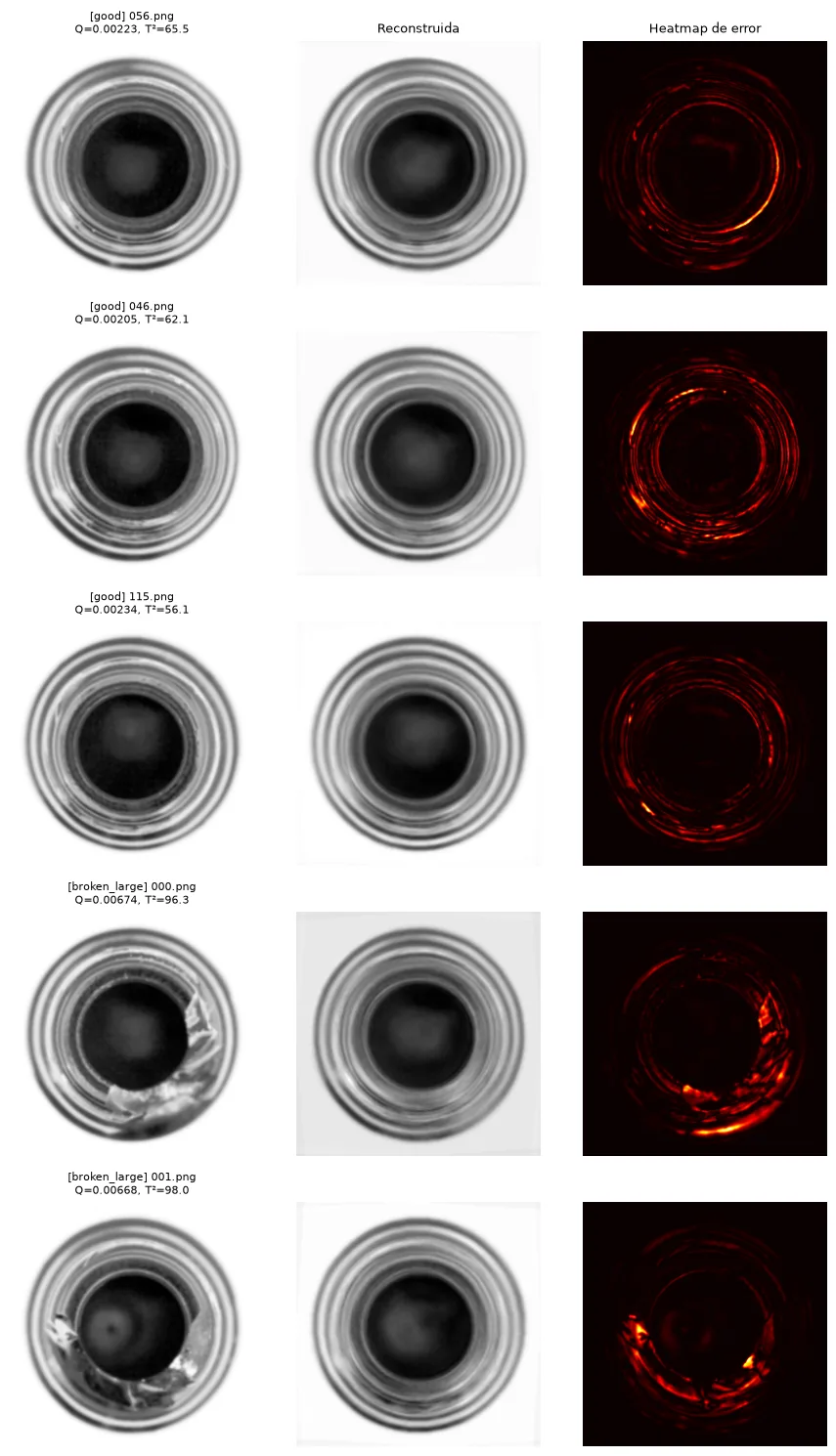
The PCA model explains itself the same way, with original, rebuild, and where the rebuild missed:

PCA flagged images: original, reconstruction and error heatmap — The first five images PCA flagged: three of its good-bottle false alarms (top), then two large breaks lighting up exactly at the damage. tap to zoom

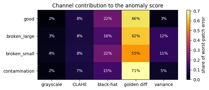
Which filter raised the neural net's alarm?

Breaking the worst tile's error down by filter shows that the golden diff (the difference from an "average good bottle" template) does most of the work, for every defect type.

Share of the alarm signal contributed by each vision filter — Share of the alarm signal by filter, averaged per defect type.

Show the notebook code: which filter raised the alarm

def channel_residuals(path):
    """Per-channel share of the worst patch's reconstruction error."""
    stack = build_channels(load_rgb(path), golden)
    Xs = torch.from_numpy(((to_patches(stack) - mean) / std).astype(np.float32)).to(DEVICE)
    model.eval()
    with torch.no_grad():
        resid = (model(Xs) - Xs).cpu().numpy()
    per_patch = np.sqrt((resid ** 2).sum(axis=1))
    worst = resid[int(np.argmax(per_patch))].reshape(PATCH, PATCH, N_CHANNELS)
    contrib = (worst ** 2).sum(axis=(0, 1))
    return contrib / contrib.sum()

From bottle_anomaly_detection.ipynb. The worst tile's rebuild error, split across the five filters. This is the classic process-monitoring question: which variable caused the alarm?

§5 · Deep-dive · the PCA dial

How many patterns does PCA need?

PCA's big setting is how many patterns to keep. Keep too few and it can't rebuild even good bottles: false alarms everywhere. Keep too many and it rebuilds defects too, and the alarm goes quiet. Drag the slider to move along the real curve from the notebook:

Reading the curve

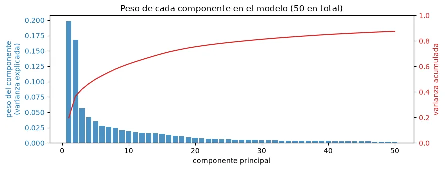
The first few patterns capture the big shapes, so the curve climbs fast, then flattens as later patterns only add fine detail. The shipped setting of 50 patterns keeps about 88% of the detail in a good-bottle photo; reaching the 95% mark would take about 113. Staying deliberately below that mark is what keeps defects poorly rebuilt, and therefore visible.

Weight of each of the 50 PCA patterns, with the cumulative total — How much each of the 50 patterns matters: the first two dominate, then the weights fall off fast; the red line is the running total. tap to zoom

Show the notebook code: the curve behind the slider

pca_exploratorio = PCA().fit(X_train)
varianza_acumulada = np.cumsum(pca_exploratorio.explained_variance_ratio_)

n_para_95 = int(np.argmax(varianza_acumulada >= 0.95)) + 1
print(f"Componentes necesarios para explicar 95% de varianza: {n_para_95}")
print(f"(estás usando N_COMPONENTS={N_COMPONENTS})")
# -> Componentes necesarios para explicar 95% de varianza: 113
# -> (estás usando N_COMPONENTS=50)

From pca_avanzado_bottle.ipynb. The real numbers behind the slider: 113 patterns would reach 95% of the detail; the shipped model deliberately stops at 50.

§6 · The harder product

The transistor line took three tries

Pointed at a fussier product (transistors, whose three metal legs shift slightly from photo to photo), the bottle recipe simply didn't transfer. It took three real attempts before good and defective scores separated. The same score-curve charts tell the story:

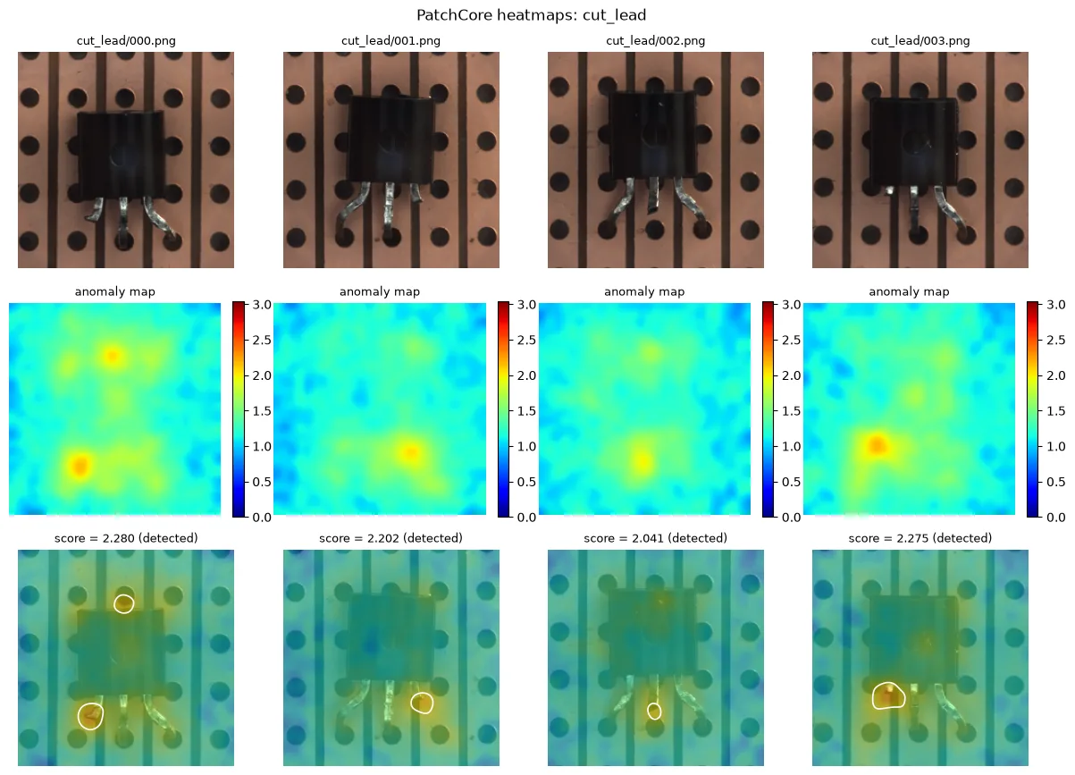
Why the third attempt won: PatchCore never rebuilds the image at all. It compares each patch against a memory bank of known-good patches, so ordinary part-to-part variation is recognised instead of punished. The product didn't get worse between attempts; it was just a harder object, and it needed a method built for subtle, local defects.

PatchCore heatmaps for four cut_lead transistor images, all flagged correctly — PatchCore on cut-lead transistors: all four flagged, with the hot spot right at the cut leg. tap to zoom