Data & the Two Models · Bottle Anomaly Detection

§1 · The setup

The data

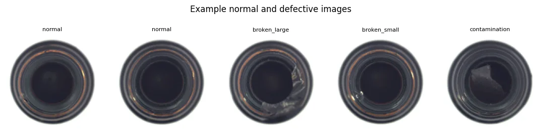
Top-down photos of a glass bottle from the MVTec AD benchmark, the standard industrial anomaly-detection dataset. Three kinds of defect exist (large breaks, small breaks and contamination), but during training the models only ever see good bottles. That's the whole point: on a real production line you have thousands of photos of good parts and almost none of defects, so a normal classifier has nothing to learn the "bad" class from.

Example normal and defective bottle images — Example good bottles and one of each defect type. tap to zoom

split	images	OK	BAD	role
train	125	125	0	learn what "normal" is
validation	41	41	0	set the alarm level
test	126	63	63	final exam, taken once

Both models use the same split, and each one's alarm level is fixed in advance using only good bottles it hadn't trained on. No defective image ever influences training or the alarm level; the test set is graded exactly once.

Why the split matters

The 41-image validation set exists for exactly one job: choosing where to put the alarm line. If you set the alarm level on the same images you trained on, the model looks unrealistically confident and the threshold lands too low; if you peek at the test set, your final score is a lie. Setting it on held-out good bottles gives a designed false-alarm rate (the 95th percentile → roughly 5% of good bottles flagged) before the model has ever seen a single defect.

§2 · The contenders

Two ways to learn "normal"

Both models work on the same idea: learn to rebuild good bottles, then flag anything they can't rebuild well. A defect is, by definition, something the model has never seen, so its rebuild of a defective photo comes out wrong, and the size of that error is the alarm signal.

Model A · PCA · built by a group member

The pattern-matcher

Even out the photo. Equalize the lighting and lightly blur, so differences in illumination don't look like defects.
Find the 50 strongest patterns shared by all good bottles (this is what PCA does; think of them as 50 "ingredients" of a normal bottle photo).
Rebuild each new photo from only those 50 ingredients, and measure two things: how much the rebuild misses (Q) and how unusual the ingredient mix is (T²).
Alarm if either number is too high.

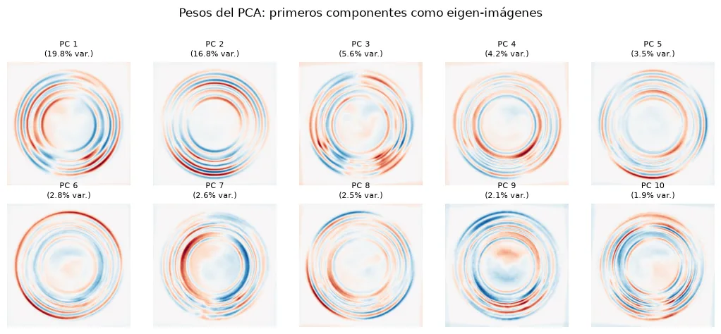
The first ten PCA patterns visualized as eigen-images — The model's learned weights, made visible: the first 10 of the 50 patterns (3.3 million numbers in total). Red = brighter than an average bottle, blue = darker. The first two alone carry 37% of what "normal" looks like. tap to zoom

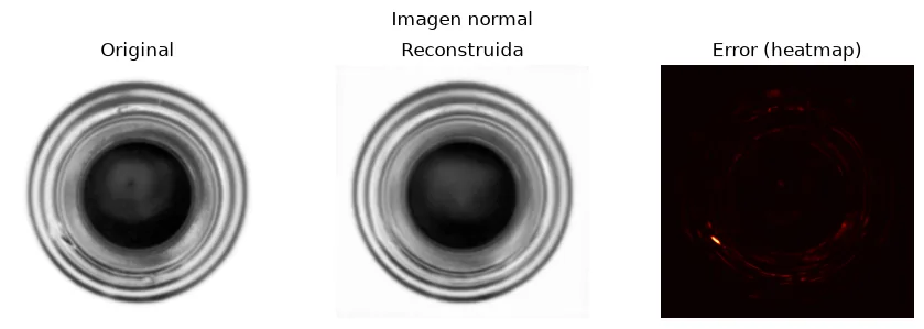
A normal bottle, its PCA reconstruction, and the difference between them — A good bottle (left), what PCA rebuilds from its 50 patterns (middle), and where the rebuild misses (right): barely anywhere. tap to zoom

Show the notebook code: the two alarms, Q and T²

def calcular_q_y_t2(X_datos, pca):
    """Q: error de reconstrucción. T2: distancia de Mahalanobis en el espacio de componentes."""
    scores = pca.transform(X_datos)               # proyección en componentes
    X_reconstruido = pca.inverse_transform(scores)

    q = np.mean((X_datos - X_reconstruido) ** 2, axis=1)

    varianzas = pca.explained_variance_
    t2 = np.sum((scores ** 2) / varianzas, axis=1)

    return q, t2

# thresholds calibrados con HOLDOUT (imágenes normales no vistas), no con train
threshold_q = np.percentile(q_holdout, THRESHOLD_PERCENTILE)
threshold_t2 = np.percentile(t2_holdout, THRESHOLD_PERCENTILE)

def es_anomalo(q_valor, t2_valor):
    """Anómalo si CUALQUIERA de los dos scores supera su threshold."""
    return (q_valor > threshold_q) or (t2_valor > threshold_t2)

From pca_avanzado_bottle.ipynb, written in Spanish by its author. Q is how much the rebuild misses; T² is how unusual the ingredient mix is. A bottle is flagged if either alarm trips.

Model B · Patch autoencoder · the neural net

The tile inspector

Run five vision filters over the photo; each one makes a different kind of flaw easier to see (tap through them below).
Cut the result into 32×32-pixel tiles, so a small chip can't hide in a big picture.
A small neural network rebuilds each tile, having squeezed it through a tiny 4-number bottleneck, so it can only memorise what normal tiles look like.
Score the bottle by its 5 worst tiles. One terrible tile (a break) or several mediocre ones (spread-out dirt) both trip the alarm.

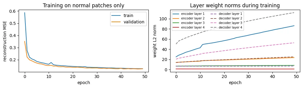
Training curve and layer weight norms of the neural network — The network learning: its rebuild error falls and levels off (left), while the weights in each layer grow and settle as it memorises what normal tiles look like (right). tap to zoom

11,674,884 parameters · trained for 50 epochs on a laptop

Show the notebook code: the network itself

class PatchAE(nn.Module):
    def __init__(self, dim=PATCH * PATCH * N_CHANNELS, bottleneck=BOTTLENECK):
        super().__init__()
        self.encoder = nn.Sequential(
            nn.Linear(dim, 1024), nn.ReLU(),
            nn.Linear(1024, 512), nn.ReLU(),
            nn.Linear(512, 128), nn.ReLU(),
            nn.Linear(128, bottleneck), nn.ReLU(),
        )
        self.decoder = nn.Sequential(
            nn.Linear(bottleneck, 128), nn.ReLU(),
            nn.Linear(128, 512), nn.ReLU(),
            nn.Linear(512, 1024), nn.ReLU(),
            nn.Linear(1024, dim),
        )

    def forward(self, x):
        return self.decoder(self.encoder(x))

From bottle_anomaly_detection.ipynb: the whole model. Each 32×32×5 tile (5,120 numbers) is squeezed through a bottleneck of just 4 numbers and rebuilt.

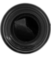
The five filters, on a real contaminated bottle

Show the notebook code: all five filters

def golden_template(paths):
    # Median of the CLAHE-equalised normals: the golden-diff channel compares
    # contrast-boosted images, which makes faint contamination stand out.
    grays = np.stack([apply_clahe(to_gray_u8(load_rgb(p))) for p in paths])
    return np.median(grays, axis=0).astype(np.uint8)

def build_channels(rgb01, golden_gray):
    gray = to_gray_u8(rgb01)
    clahe = apply_clahe(gray)
    k = max(5, IMAGE_SIZE // 16) | 1
    kernel = cv2.getStructuringElement(cv2.MORPH_ELLIPSE, (k, k))
    blackhat = cv2.morphologyEx(gray, cv2.MORPH_BLACKHAT, kernel)
    gdiff = np.abs(clahe.astype(np.float32) - golden_gray.astype(np.float32))
    g = gray.astype(np.float32) / 255.0
    mu = cv2.boxFilter(g, -1, (9, 9))
    mu2 = cv2.boxFilter(g * g, -1, (9, 9))
    local_std = np.sqrt(np.clip(mu2 - mu * mu, 0, None))
    return np.dstack([
        g[..., None],
        clahe.astype(np.float32) / 255.0,
        blackhat.astype(np.float32) / 255.0,
        gdiff / 255.0,
        np.clip(local_std * 4.0, 0.0, 1.0),
    ]).astype(np.float32)

From bottle_anomaly_detection.ipynb. The five filters in one function: grayscale, CLAHE, black-hat, the golden diff against a median template, and local variance.